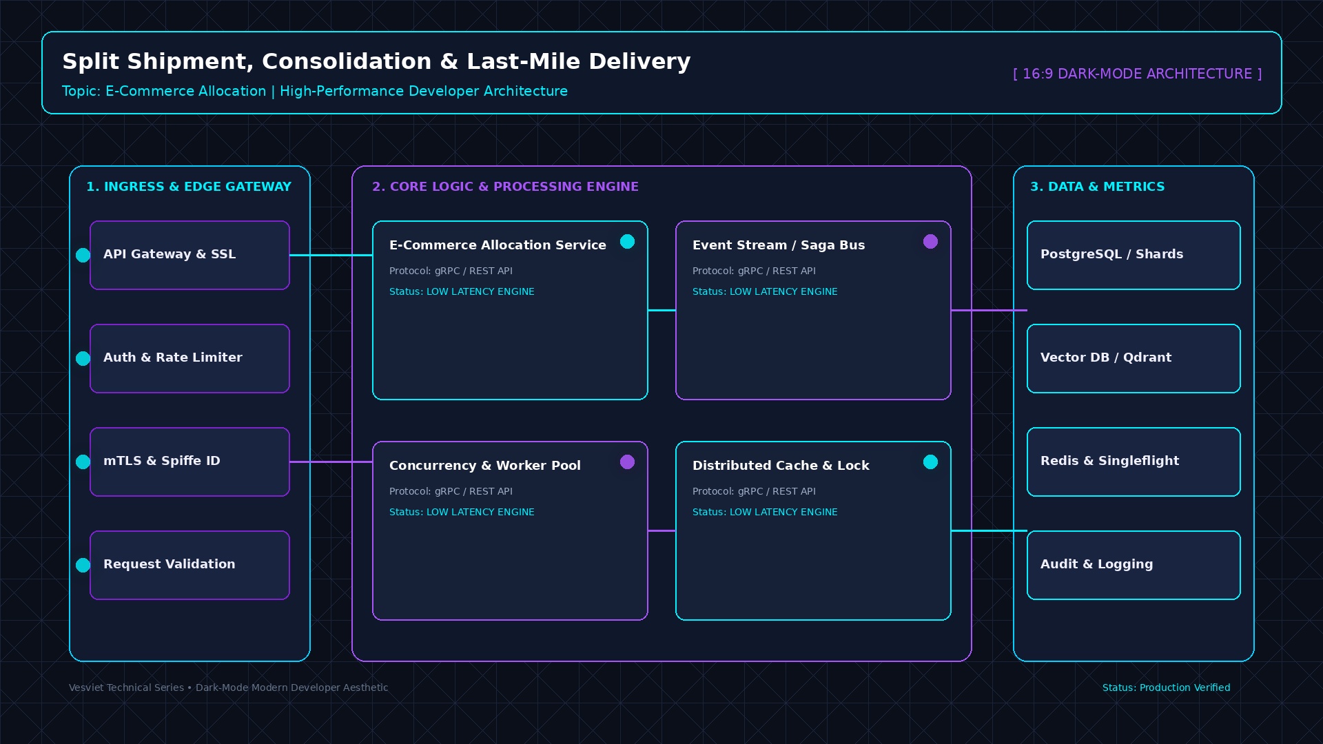
Order Fulfillment Algorithm: Warehouse to Last-Mile

Executive Summary & Fulfillment Fundamentals

When an order is confirmed, the fulfillment system executes a multi-step decision pipeline:

1. Available-to-Promise (ATP) Check: Filter candidate warehouses by real-time uncommitted stock.
2. Cost & Proximity Scoring: Evaluate shipping distance, labor rate, carrier capacity, and SLA risk.
3. Split vs. Consolidate Trade-Off: Determine whether to ship from multiple warehouses or wait for inventory consolidation.
4. CONDOR & Anticipatory Dispatch: Pre-position stock globally based on probabilistic ML demand forecasts.
5. Last-Mile VRP Solving: Optimize driver routes using vehicle routing solvers (OR-Tools / GraphHopper).

Step 1 — Real-Time Inventory & Available-to-Promise (ATP)

Physical stock on hand does not equal sellable stock. Fulfillment systems distinguish between raw inventory counts and uncommitted inventory:

• Physical On-Hand: Total inventory units located inside the warehouse bin.
• Available-to-Promise (ATP): Physical stock minus hard-committed and soft-reserved units.

Soft Reservations with TTL

When a customer enters checkout, a soft reservation decrements ATP in an in-memory Redis cluster. The reservation carries a TTL (typically 5–15 minutes). If payment fails or the session times out, the reservation automatically expires and ATP is restored.

Production Redis Lua Engine for Atomic ATP Soft Reservations

In high-concurrency e-commerce environments during sales events, naive non-atomic stock checks (e.g., executing a read GET stock followed by DECRBY) cause catastrophic race conditions and overselling. To prevent database row lock contention while maintaining strict transactional guarantees, modern order fulfillment engines delegate soft reservations to single-threaded, atomic Redis Lua scripts.

Atomic Reservation Protocol:

1. Stock Check & Decrement: Atomically verify if stock_key (e.g., atp:wh_sg01:sku_9942) holds sufficient uncommitted units.
2. TTL Key Binding: If stock is available, decrement stock_key by requested_qty and create a reservation key (reservation:ord_1042:sku_9942) bound with a strict Time-To-Live (TTL) expiration window (e.g., 900 seconds / 15 minutes).
3. Rollback & Expire: If stock is insufficient, exit immediately with zero mutations. If checkout completes, the worker converts the soft reservation into a hard database commitment. If the session expires, Redis keyspace notifications (__keyevent@0__:expired) automatically trigger an INCRBY rollback back to the warehouse stock pool.

Thread-safe Go implementations execute atomic soft reservations using github.com/redis/go-redis/v9:

package main

import (
	"context"
	"fmt"
	"time"

	"github.com/redis/go-redis/v9"
)

// AtomicLuaReserve evaluates available stock, decrements counter, and sets TTL reservation atomically.
const AtomicLuaReserve = `
local stock_key = KEYS[1]
local res_key   = KEYS[2]
local req_qty   = tonumber(ARGV[1])
local ttl_sec   = tonumber(ARGV[2])

local current_stock = tonumber(redis.call("GET", stock_key) or "0")
if current_stock >= req_qty then
    redis.call("DECRBY", stock_key, req_qty)
    redis.call("SETEX", res_key, ttl_sec, req_qty)
    return 1
else
    return 0
end
`

type InventoryEngine struct {
	client *redis.Client
	script *redis.Script
}

// NewInventoryEngine initializes the Redis client and pre-compiles the Lua script SHA.
func NewInventoryEngine(client *redis.Client) *InventoryEngine {
	return &InventoryEngine{
		client: client,
		script: redis.NewScript(AtomicLuaReserve),
	}
}

// ReserveATP executes the atomic soft reservation for an order SKU.
func (e *InventoryEngine) ReserveATP(ctx context.Context, warehouseID, sku, orderID string, qty int, ttl time.Duration) (bool, error) {
	stockKey := fmt.Sprintf("atp:{%s:%s}:stock", warehouseID, sku)
	resKey := fmt.Sprintf("atp:{%s:%s}:res:%s", warehouseID, sku, orderID)

	keys := []string{stockKey, resKey}
	args := []interface{}{qty, int(ttl.Seconds())}

	res, err := e.script.Run(ctx, e.client, keys, args...).Int64()
	if err != nil {
		return false, fmt.Errorf("redis ATP reservation script failed: %w", err)
	}

	return res == 1, nil
}

Step 2 — Warehouse Selection Cost Function

The allocation engine evaluates candidate warehouses using a multi-criteria objective function:

$$\text{Cost}(W, O) = (d \cdot r_{\text{carrier}}) + c_{\text{labor}} + P_{\text{SLA}} + S_{\text{capacity}} - B_{\text{eco}}$$

Where:

• $d$: Distance from warehouse $W$ to delivery destination
• $r_{\text{carrier}}$: Carrier rate per km
• $c_{\text{labor}}$: Warehouse pick/pack labor cost per unit
• $P_{\text{SLA}}$: Penalty score if fulfillment time risks missing delivery window
• $S_{\text{capacity}}$: Carrier surcharge when daily outbound volume exceeds 85% capacity
• $B_{\text{eco}}$: Eco-bonus for green fulfillment locations

Step 3 — Amazon CONDOR & Constraint Optimization

Amazon’s CONDOR system operates at a global fleet level above per-order routing logic to prevent regional inventory stockouts:

• Inputs: Real-time ATP across all fulfillment centers, historical demand signals, regional ML demand forecasts (14-day window), carrier contract tiers.
• Outputs: Proactive inventory transfer recommendations (rebalancing stock from central FCs to regional sortation centers before orders are placed).

Step 4 — Anticipatory & Predictive Shipping

Anticipatory shipping uses predictive ML models (browsing patterns, wishlist items, regional trends) to ship high-probability items to regional hub centers before the customer places the order. When the order occurs, the package is already in the buyer’s metro area, enabling same-day delivery at minimal expedited freight cost.

Step 5 — Split Shipment vs. Consolidation Logic

Step 6 — Last-Mile Vehicle Routing Problem (VRP) Solver

The last-mile dispatch system solves a Capacitated Vehicle Routing Problem (CVRP) with Time Windows. Beyond simple distance minimization, enterprise logistics engines enforce physical fleet payload capacity limits and node disjunctions (penalizing dropped stops during capacity overflow) to prevent dispatch deadlocks.

Production Google OR-Tools VRP Solver Parameter Configuration

Production last-mile dispatch engines optimize multi-vehicle delivery routes by configuring Google OR-Tools pywrapcp with Guided Local Search metaheuristics:

from typing import Dict, List, Tuple
from ortools.constraint_solver import routing_enums_pb2, pywrapcp

def solve_capacitated_vrp(
    distance_matrix: List[List[int]],
    demands: List[int],
    vehicle_capacities: List[int],
    depot: int = 0,
    time_limit_sec: int = 15,
) -> Tuple[Dict[int, List[int]], int]:
    """Solves Capacitated VRP with payload limits, drop penalties, and GLS metaheuristics."""
    num_locations = len(distance_matrix)
    num_vehicles = len(vehicle_capacities)

    # 1. Initialize Routing Manager and Model
    manager = pywrapcp.RoutingIndexManager(num_locations, num_vehicles, depot)
    routing = pywrapcp.RoutingModel(manager)

    # 2. Distance Callback Registration
    def distance_callback(from_index: int, to_index: int) -> int:
        from_node = manager.IndexToNode(from_index)
        to_node = manager.IndexToNode(to_index)
        return distance_matrix[from_node][to_node]

    transit_idx = routing.RegisterTransitCallback(distance_callback)
    routing.SetArcCostEvaluatorOfAllVehicles(transit_idx)

    # 3. Add Capacity Constraint Dimension
    def demand_callback(from_index: int) -> int:
        from_node = manager.IndexToNode(from_index)
        return demands[from_node]

    demand_idx = routing.RegisterUnaryTransitCallback(demand_callback)
    routing.AddDimensionWithVehicleCapacity(
        demand_idx,
        0,                  # Null capacity slack
        vehicle_capacities, # Vehicle payload limit vector
        True,               # Start capacity accumulator at zero
        "Capacity"
    )

    # 4. Enforce Node Disjunctions with Overflow Penalty
    penalty = 100_000  # Penalty for unserviced drop point
    for node in range(1, num_locations):
        routing.AddDisjunction([manager.NodeToIndex(node)], penalty)

    # 5. Search Parameter Tuning & Metaheuristics
    search_params = pywrapcp.DefaultRoutingSearchParameters()
    search_params.first_solution_strategy = (
        routing_enums_pb2.FirstSolutionStrategy.PATH_CHEAPEST_ARC
    )
    search_params.local_search_metaheuristic = (
        routing_enums_pb2.LocalSearchMetaheuristic.GUIDED_LOCAL_SEARCH
    )
    search_params.time_limit.seconds = time_limit_sec
    search_params.log_search = False

    # 6. Solve and Extract Vehicle Route Vectors
    solution = routing.SolveWithParameters(search_params)
    if not solution:
        return {}, -1

    routes: Dict[int, List[int]] = {}
    for vehicle_id in range(num_vehicles):
        index = routing.Start(vehicle_id)
        route = []
        while not routing.IsEnd(index):
            node = manager.IndexToNode(index)
            route.append(node)
            index = solution.Value(routing.NextVar(index))
        route.append(manager.IndexToNode(index))
        routes[vehicle_id] = route

    return routes, solution.ObjectiveValue()

Key Solver Design Decisions:

• First Solution Strategy (PATH_CHEAPEST_ARC): Rapidly constructs an initial feasible route baseline to maximize search efficiency within tight latency budgets.
• Guided Local Search (GUIDED_LOCAL_SEARCH): Escapes local minima by dynamically penalizing frequently traversed solution edges during local transformations.
• Disjunction Penalties (AddDisjunction): Guarantees solver feasibility when total daily demand exceeds available driver fleet capacity by isolating unserved nodes for 3PL fallback dispatch.

Frequently Asked Questions

How do e-commerce algorithms determine which warehouse fulfills an order?

Warehouse selection algorithms evaluate candidate fulfillment centers using a multi-criteria cost function combining shipping distance, carrier transit rates, labor costs, SLA risk penalties, and real-time Available-to-Promise (ATP) stock. Distributed optimization systems continuously rebalance global inventory to prevent local stockouts and minimize split shipments.

What is the Vehicle Routing Problem (VRP) in last-mile logistics?

The Vehicle Routing Problem is a combinatorial optimization challenge that calculates optimal delivery routes for a fleet servicing customer locations. Solvers like Google OR-Tools apply vehicle capacity dimensions, time-window constraints, and drop penalties to minimize total transit distance while maintaining delivery SLAs.

How does Amazon’s anticipatory shipping model reduce delivery latency?

Anticipatory shipping utilizes machine learning demand forecasts to transport high-probability items to regional fulfillment hubs before customers complete their purchases. Once an order is placed, the package is already positioned in the destination metro area, enabling same-day delivery at standard shipping rates.

Related Reading

• GraphHopper Distance Matrix: Self-Host, API & Alternatives — producing the cost matrix the VRP solver consumes.
• OSRM vs GraphHopper: Routing Engine Comparison — choosing the routing engine behind last-mile optimization.
• Real-Time Inventory: Kafka, CDC & Redis — the Available-to-Promise stock signal driving warehouse selection.
• Surge Pricing & Spatial Indexing Architecture — H3 spatial indexing applied to demand-side pricing.